Chapter 7 Binomial Logistic Regression
Chapter 6 Learning Outcomes
State the assumptions associated with a binomial logistic regression model and determine whether the assumptions are satisfied.
Calculate probabilities and odds and expected changes associated with fixed effects in a binomial logistic regression model.
Interpret fixed effect coefficients in a binomial logistic regression model.
Analyze data using a binomial logistic regression model and Zero-Inflated Poisson Model in R.
Interpret fixed effect coefficients in a Zero-Inflated Poisson model.
Explain the role of a link function in a generalized linear model and determine which link function(s) might be appropriate in a given model.
These notes provide a summary of Chapter 6 in Beyond Multiple Linear Regression by Roback and Legler. The dataset we work with is different than those in the text, but much of the code and analysis is based off the examples in the text. Github repository.
# Packages required for Chapter 6
library(gridExtra)
library(mnormt)
library(lme4)
library(knitr)
library(pander)
library(tidyverse)
library(gridExtra)
library(corrplot)
library(openintro)
7.1 Binomial Logistic Regression
7.1.1 Binary Response Data
We can use logistic regression to model binary responses, such as whether or not a student person defaults on a credit card payment, as in the dataset below.
In this dataset, each row represents an individual with a single yes/no response.
##   default student   balance    income
## 1      No      No  729.5265 44361.625
## 2      No     Yes  817.1804 12106.135
## 3      No      No 1073.5492 31767.139
## 4      No      No  529.2506 35704.494
## 5      No      No  785.6559 38463.496
## 6      No     Yes  919.5885  7491.559
7.1.2 Binomial Response Data
We can also use logistic regression to model data where the rows represent the number of “successes” in a fixed number of trials.
For example:
- Number of games won by a sports team in a given number of games.
- Number of people who survive for at least 10 years after being diagnosed with a disease.
- Number of people who vote for a candidate in election our of total number of voters.
We’ll refer to this kind of regression as Binomial Logistic Regression, though the term logistic regression is used somewhat ambiguously and is sometimes applied to this context as well.
7.1.3 Challenger O-Rings Data
In 1986, the space shuttle Challenger exploded just 73 seconds into flight, killing all seven crew members. The disaster is believed to have been caused by damage to a seal called an O-ring that likely occurred during takeoff. Damage to O-rings is believed to be related to ambient temperature during launch.
At the time of the launch, the temperature was only 31 degrees Fahrenheit, which is very cold for shuttle launches.
Shown below are data for 23 other shuttle missions, including the temperature (in degrees Fahrenheit) at the time of launch and the number of damaged and undamaged O-rings, out of six total O-rings.
| mission | temperature | damaged | undamaged |
|---|---|---|---|
| 1 | 53 | 5 | 1 |
| 2 | 57 | 1 | 5 |
| 3 | 58 | 1 | 5 |
| 4 | 63 | 1 | 5 |
| 5 | 66 | 0 | 6 |
| 6 | 67 | 0 | 6 |
| 7 | 67 | 0 | 6 |
| 8 | 67 | 0 | 6 |
| 9 | 68 | 0 | 6 |
| 10 | 69 | 0 | 6 |
| 11 | 70 | 1 | 5 |
| 12 | 70 | 0 | 6 |
| 13 | 70 | 1 | 5 |
| 14 | 70 | 0 | 6 |
| 15 | 72 | 0 | 6 |
| 16 | 73 | 0 | 6 |
| 17 | 75 | 0 | 6 |
| 18 | 75 | 1 | 5 |
| 19 | 76 | 0 | 6 |
| 20 | 76 | 0 | 6 |
| 21 | 78 | 0 | 6 |
| 22 | 79 | 0 | 6 |
| 23 | 81 | 0 | 6 |
We plot percentage damaged by temperature. Shown are a linear regression line, and a logistic regression curve.
ggplot(data=orings, aes(x=temperature, y=damaged/(damaged+undamaged))) + geom_point() + geom_smooth(method="lm", se=FALSE, color="green")  +
  stat_smooth(method="glm", se=FALSE, method.args = list(family=binomial))
7.1.4 Modeling Number Damaged
We know that there are a total of 6 O-rings on a shuttle. Suppose we knew the probability of an individual O-ring being damaged at a given temperature.
Since the response is a count, we might think to use a Poisson distribution. However, a Poisson distribution does not place an upper bound on the number damaged O-rings. This is unrealistic since we know that in reality, we cannot have more than 6 damaged O-rings.
7.1.5 The Binomial Distribution
A Binomial random variable is a discrete random variable that models the number of “successes” in a fixed number of independent trials. We let \(n\) represent the number of trials, and \(p\) represent the probability of success on any given trial.
Notation: \(Y\sim Binom(n,p)\), Probability Mass Function: \(\text{P}(Y=y) = {n\choose y}p^y(1-p)^{n-y}\)
For \(n = 6, p=0.6\),
\[ Pr(Y=0) = {6\choose 0}0.6^0(0.4)^{6} = 1(0.4)^6\approx(0.004) \]
\[ Pr(Y=1) = {6\choose 1}0.6^1(0.4)^{5} = 6(0.6)(0.4)^5\approx(0.006) \]
\[ Pr(Y=2) = {6\choose 2}0.6^2(0.4)^{4} = 15(0.6)^2(0.4)^4\approx(0.1382) \]
\[ Pr(Y=3) = {6\choose 3}0.6^3(0.4)^{3} = 20(0.6)^3(0.4)^3\approx(0.2765) \]
\[ Pr(Y=4) = {6\choose 4}0.6^4(0.4)^{2} = 15(0.6)^4(0.4)^2\approx(0.3110) \]
\[ Pr(Y=5) = {6\choose 5}0.6^5(0.4)^{1} = 6(0.6)^5(0.4)^1\approx(0.1866) \]
\[ Pr(Y=5) = {6\choose 6}0.6^6(0.4)^{0} = 1(0.6)^6(0.4)^0\approx(0.0467) \]
In a binomial distribution, the mean is \(np\),
and the variance is \(np(1-p)\).
A binomial distribution with \(n=1\) is called a Bernoulli Distribution, denoted \(Ber(p)\).
7.1.6 Binomial Distribution for \(n=6, p=0.6\)
df <- data.frame(x = 0:6, y = dbinom(0:6, size = 6, prob=0.6))
ggplot(df, aes(x = x, y = y)) + geom_bar(stat = "identity", col = "white", fill = "blue") +
  scale_y_continuous(expand = c(0.01, 0)) + scale_x_continuous(breaks=(0:6)) + xlab("x") + ylab(expression(paste("p(x|", p, ")"))) + ggtitle("n=6, p=0.6") + theme_bw() +
  theme(plot.title = element_text(size = rel(1.2), vjust = 1.5))
Mean = \(0.6 \times 6=3.6\)
Variance = \(6\times 0.6 \times 0.4=1.44\)
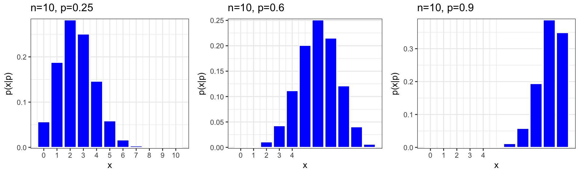
7.1.7 More Binomial Distributions
We plot binomial distributions with \(n=10\), \(p=0.25, 0.6, 0.9\)
7.1.8 Connecting Expected Response to Explatory Variables
set.seed(0)
dat <- tibble(x=runif(200, -5, 10),
                  p=exp(-2+1*x)/(1+exp(-2+1*x)),
                  y=rbinom(200, 1, p),
                  y2=.3408+.0901*x,
                  logit=log(p/(1-p)))
dat2 <- tibble(x = c(dat$x, dat$x),
               y = c(dat$y2, dat$p),
               `Regression model` = c(rep("linear", 200),
                                      rep("logistic", 200)))
ggplot() +
  geom_point(data = dat, aes(x, y)) +
  geom_line(data = dat2, aes(x, y, linetype = `Regression model`))  + ylab("p")
Let \(p_i\) represent the probability that an individual O-ring on mission i was damaged.
We want to connect \(p_i\) to our explanatory variable, temperature.
Assuming
\[p_i = \beta_0+\beta_1X_{1} + \ldots + \beta_pX_p\]
is a bad idea since \(p_1\) must stay between -1 and 1.
We’ll use a sigmoidal function of the form
\[p_i = \frac{e^{\beta_0+\beta_1X_{1} + \ldots + \beta_pX_p}}{1+e^{\beta_0+\beta_1X_{1} + \ldots + \beta_pX_p}}\]
Equivalently:
\[\text{log}\left(\frac{{p_i}}{{1-p_i}}\right) = \beta_0+\beta_1X_{1} + \ldots + \beta_pX_p \]
The function \(\text{log}\left(\frac{{p_i}}{{1-p_i}}\right)\) is called \(\text{logit}(p_i)\). So, we can say:
\[\text{logit}(p_i) = \beta_0+\beta_1X_{i1} + \ldots + \beta_pX_{ip}\]
The function \(f(p) = \text{logit}(p) = log\left(\frac{p}{1-p}\right)\) is the link function.
Note: we could use different functions that map the real numbers into the interval (0,1), but the logit function works well and is frequently used.
7.1.9 Odds and Odds Ratio
For an event with probability \(p\), the odds of the event occuring are \(\frac{p}{1-p}\)
For two events \(p_1\) and \(p_2\) the odds ratio is defined as \(\frac{\text{Odds of Event 1}}{\text{Odds of Event 1}} = \frac{\frac{p_1}{1-p_1}}{\frac{p_2}{1-p_2}}\)
7.1.10 Interpreting Regression Coefficients
Let’s suppose we have one explanatory variable \(x\), so
\[p_i = \frac{e^{\beta_0+\beta_1X_{1}}}{1+e^{\beta_0+\beta_1X_{1}}}, \]
Consider the odds ratio for a case \(j\) with explanatory variable \(x + 1\), compared to case \(i\) with explanatory variable \(x\).
That is \(\text{log}\left(\frac{p_i}{1-p_i}\right) = \beta_0+\beta_1x\), and \(\text{log}\left(\frac{p_j}{1-p_j}\right) = \beta_0+\beta_1(x+1)\).
\(\text{log}\left(\frac{\frac{p_j}{1-p_j}}{\frac{p_i}{1-p_i}}\right)=\text{log}\left(\frac{p_j}{1-p_j}\right)-\text{log}\left(\frac{p_i}{1-p_j}\right)=\beta_0+\beta_1(x+1)-(\beta_0+\beta_1(x))=\beta_1.\)
For each 1-unit increase in \(x\) the log of the odds ratio of success to failure is expected to multiply by a factor of \(\beta_1\).
For each 1-unit increase in \(x\) the odds ratio of success to failure is expected to multiply by a factor of \(e^{\beta_1}\).
For a categorical variable \(x_j\) the odds success to failure in category \(j\), are expected to be \(e^{\beta_1}\) times higher in category \(j\) than in the baseline category.
7.1.11 Binomial Logistic Regression Assumptions
A logistic regression model relies on the following assumptions:
- Binary Response The response variable is dichotomous (two possible responses) or the sum of dichotomous responses.
- Independence The observations must be independent of one another.
- Variance Structure By definition, the variance of a binomial random variable is \(np(1-p)\), so that variability is highest when \(p=.5\).
- Linearity The log of the odds ratio, \(\text{log}(\frac{p}{1-p}) = \text{logit}(p)\), must be a linear function of \(x\).
7.2 Model for Challenger Disaster O-rings
7.2.1 Binomial Logistic Model for O-rings
M1 <- glm(cbind(damaged, undamaged) ~ temperature , family = binomial(link="logit"), data = orings)
summary(M1)
##
## Call:
## glm(formula = cbind(damaged, undamaged) ~ temperature, family = binomial(link = "logit"),
## data = orings)
##
## Coefficients:
## Estimate Std. Error z value Pr(>|z|)
## (Intercept) 11.66299 3.29626 3.538 0.000403 ***
## temperature -0.21623 0.05318 -4.066 0.0000478 ***
## ---
## Signif. codes: 0 '***' 0.001 '**' 0.01 '*' 0.05 '.' 0.1 ' ' 1
##
## (Dispersion parameter for binomial family taken to be 1)
##
## Null deviance: 38.898 on 22 degrees of freedom
## Residual deviance: 16.912 on 21 degrees of freedom
## AIC: 33.675
##
## Number of Fisher Scoring iterations: 6For each one degree increase in temperature, the odds of damage to the O-ring are expected to multiply by a factor of \(exp{-0.216}\approx0.80555\). That is, for each one-degree increase in temperature, odds of damage are expected to decrease by 20%.
If the temperature is 55 degrees, the probability of an individual O-ring being damaged is:
\[\frac{e^{11.66 - 0.216\times 55}}{1+ e^{11.66 - 0.216\times 55}}=0.445\]
If the temperature is 75 degrees, the probability of an individual O-ring being damaged is:
\[\frac{e^{11.66 - 0.216\times 75}}{1+ e^{11.66 - 0.216\times 75}}=0.01\]
If the temperature is 31 degrees, the probability of an individual O-ring being damaged is:
\[\frac{e^{11.66 - 0.216\times 31}}{1+ e^{11.66 - 0.216\times 31}}=0.99\]
This is an extrapolation, but should be enough to raise serious concern.
7.2.2 Checking Linearity Assumption
The model assumes that \(\text{log}\left(\frac{p}{1-p}\right) = \text{logit}(p)\) is a linear function of \(x\). To check this, we calculate \(\hat{p}_i\), the proportion of damaged o-rings for each mission and plot \(\text{log}\left(\frac{\hat{p}_i}{1-\hat{p_i}}\right)\) (this quantity is called the empirical logit) against temperature.
When there are counts with 0’s (presenting problems when taking log), it is common to add 1 “success” and 1 “failure” before calculating the empirical logit.
phat <- with(orings, (1 + damaged)/( 2 + damaged+undamaged))
orings$elogit <- log(phat/(1-phat))
## Plots
ggplot(orings, aes(x=temperature, y=elogit))+
    geom_point(shape=1) +    # Use hollow circles
    geom_smooth(method=lm,   # Add linear regression line
                se=FALSE) + # Don't add shaded confidence region
  xlab("Temperature") + ylab("empirical logits") +
  labs(title="O-Rings Empirical logits by Temperature")
Ideally, this plot would look linear. It doesn’t look great here, so we might consider using a nonlinear function of temperature inside the binomial logit model. Then again, there aren’t that many points, and a more complicated model would be harder to interpret, so let’s stick with the linear function of temperature inside the binomial logit model.
7.2.3 Overdispersion in Binomial Counts
The binomial model assumes that the variance is equal to \(np(1-p)\). Checking this using graphs or tables is often challenging. Here, we would need to group together missions with similar temperatures and calculate the variance in number of damaged O-rings between groups, and see how this compares to the expected variance \(n\hat{p}(1-\hat{p})\).
We’ll group by 5-degree temperature intervals.
summarize <- dplyr::summarize

orings <- orings |> mutate(Cuts = cut(orings$temperature,
           breaks=c(50, 55, 60, 65, 70, 75, 80, 85)))  # break points for temperature groups

oringsGrps <- orings %>% group_by(Cuts) %>%
  summarize(Nmissions = n(),
            phat = sum(damaged)/sum(damaged + undamaged),
            Obs_Var = var(damaged),
            Theoretical_Variance = 6*phat*(1-phat))
oringsGrps
## # A tibble: 7 × 5
## Cuts Nmissions phat Obs_Var Theoretical_Variance
## <fct> <int> <dbl> <dbl> <dbl>
## 1 (50,55] 1 0.833 NA 0.833
## 2 (55,60] 2 0.167 0 0.833
## 3 (60,65] 1 0.167 NA 0.833
## 4 (65,70] 10 0.0333 0.178 0.193
## 5 (70,75] 4 0.0417 0.25 0.240
## 6 (75,80] 4 0 0 0
## 7 (80,85] 1 0 NA 0In groups with 4 or more missions, the observed variance seems pretty close to the theoretical variance. Then again, there are only 3 such groups, so it’s hard to tell.
We can further test for overdispersion using Pearson residuals, as we did in Poisson regression.
7.2.4 Residuals for Binomial Logistic Regression
We examine two kinds of residuals that are similar to those we saw in Poisson regression.
Pearson Residual:
\[ \begin{equation*} \textrm{Pearson residual}_i = \frac{\textrm{actual count}-\textrm{predicted count}}{\textrm{SD of count}} = \frac{Y_i-m_i\hat{p_i}}{\sqrt{m_i\hat{p_i}(1-\hat{p_i})}} \end{equation*} \]
where \(m_i\) is the number of trials for the \(i^{th}\) observation and \(\hat{p}_i\) is the estimated probability of success for that same observation.
Deviance Residual: \[ \begin{equation*} \textrm{d}_i = \textrm{sign}(Y_i-m_i\hat{p_i})\sqrt{2[Y_i \log\left(\frac{Y_i}{m_i \hat{p_i}}\right)+ (m_i - Y_i) \log\left(\frac{m_i - Y_i}{m_i - m_i \hat{p_i}}\right)]} \end{equation*} \]
When the number of trials is large for all of the observations and the models are appropriate, both sets of residuals should follow a standard normal distribution.
7.2.5 Quasi-Binomial Model
Like in Poisson regression, we can address overdispersion by fitting quasi-binomial model that estimates a dispersion parameter \(\hat{\phi}=\frac{\sum(\textrm{Pearson residuals})^2}{n-p}\) and multiplies standard error by \(\sqrt{\phi}\).
M1b <- glm(cbind(damaged, undamaged) ~ temperature , family = quasibinomial(link="logit"), data = orings)
summary(M1b)
##
## Call:
## glm(formula = cbind(damaged, undamaged) ~ temperature, family = quasibinomial(link = "logit"),
## data = orings)
##
## Coefficients:
## Estimate Std. Error t value Pr(>|t|)
## (Intercept) 11.66299 3.81077 3.061 0.00594 **
## temperature -0.21623 0.06148 -3.517 0.00205 **
## ---
## Signif. codes: 0 '***' 0.001 '**' 0.01 '*' 0.05 '.' 0.1 ' ' 1
##
## (Dispersion parameter for quasibinomial family taken to be 1.336542)
##
## Null deviance: 38.898 on 22 degrees of freedom
## Residual deviance: 16.912 on 21 degrees of freedom
## AIC: NA
##
## Number of Fisher Scoring iterations: 6The estimate of the dispersion parameter \(\hat{\phi} = 1.336\) is not too large, confirming that overdispersion is not too much of a concern here.
Notice that standard errors, z-scores, and p-values for the quasi-binomial model were similar to those we saw in the binomial model.
Wald test statistics and p-values for all variables provide evidence of a relationship between temperature and probability of damage to an o-ring.
7.2.6 Deviance Residual Plot
We plot deviance residuals against the predicted values and against our explanatory variables to test for lack of fit.
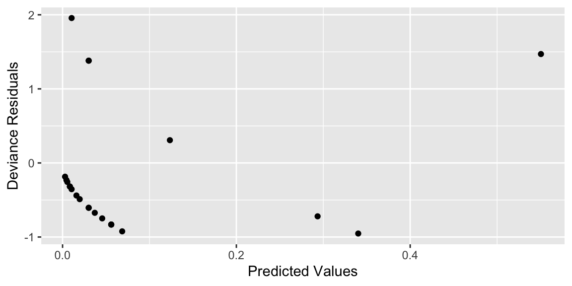
Again, we see some concerns about the linearity assumption, but we’ll stick with this model for the reasons discussed previously.
7.2.7 LLSR vs Binomial Logistic Regression
\[\begin{gather*} \underline{\textrm{Response}} \\ \mathbf{LLSR:}\textrm{ normal} \\ \mathbf{Binomial\ Regression:}\textrm{ number of successes in n trials} \\ \textrm{ } \\ \underline{\textrm{Variance}} \\ \mathbf{LLSR:}\textrm{ equal for each level of}\ X \\ \mathbf{Binomial\ Regression:}\ np(1-p)\textrm{ for each level of}\ X \\ \textrm{ } \\ \underline{\textrm{Model Fitting}} \\ \mathbf{LLSR:}\ \mu=\beta_0+\beta_1x \textrm{ using Least Squares}\\ \mathbf{Binomial\ Regression:}\ \log\left(\frac{p}{1-p}\right)=\beta_0+\beta_1x \textrm{ using Maximum Likelihood}\\ \textrm{ } \\ \underline{\textrm{EDA}} \\ \mathbf{LLSR:}\textrm{ plot $X$ vs. $Y$; add line} \\ \mathbf{Binomial\ Regression:}\textrm{ find $\log(\textrm{odds})$ for several subgroups; plot vs. $X$} \\ \end{gather*}\]
\[\begin{gather*} \underline{\textrm{Comparing Models}} \\ \mathbf{LLSR:}\textrm{ extra sum of squares F-tests; AIC/BIC} \\ \mathbf{Binomial\ Regression:}\textrm{ drop-in-deviance tests; AIC/BIC} \\ \textrm{ } \\ \underline{\textrm{Interpreting Coefficients}} \\ \mathbf{LLSR:}\ \beta_1=\textrm{ change in mean response for unit change in $X$} \\ \mathbf{Binomial\ Regression:}\ e^{\beta_1}=\textrm{ percent change in odds for unit change in $X$} \end{gather*}\]
7.3 Maximum Likelihood Estimation
7.3.1 Parameter Estimation
Recall that in ordinarly least squares regression, the estimates \(b_1, b_2, \ldots, b_p\) of regression coefficients \(\beta_1, \beta_2, \ldots \beta_p\) are chosen in a way that minimizes \(\displaystyle\sum_{i=1}^n(y_i-\hat{y_i})^2=\displaystyle\sum_{i=1}^n(y_i-(b_0+b_1x_{i1}+\ldots b_px_{ip}))^2\).
The validity of the least-squares regression process depends on the assumptions associated with a LLSR model, making it inappropriate for the kinds of models we’ve seen in this class (mixed effects models, generalized linear models, etc.). Instead, we use a process called maximum likelihood estimation.
In fact, in an ordinary LLSR model, it can be shown that maximum likelihood estimation would produce the same estimates as least squares estimation.
In this section, we’ll work through a simple example to illustrate how maximum likelihood works in a logistic regression model.
7.3.2 Steph Curry 3-Point Shooting
Stephen Curry of the Golden State Warriors is widely considered to be the best 3-point shooter in the NBA. So far during the current 2021-22 NBA season, Curry has made 251 out of 663 attempted 3 point shots (37.9%).
When playing at home, he has made 150 out of 397 3-point shots (37.8%).
When playing away, he has made 101 out of 266 4-point shots (38.0%).
We’ll use a logistic regression model to estimate the probability of Curry making a shot at home or away and test whether there is evidence of differences in his shooting based on location.
7.3.3 Model for Curry’s Shooting
We’ll start with a very simple intercept-only model. This model assumes that Curry has a constant probability of success on any shot (\(p\)), which is the same, regardless of where he is playing.
Our goal is to estimate \(p\) and to find a confidence interval for the range \(p\) could plausibly lie in.
7.3.4 Likelihood Function
A likelihood function is a function that tells us how likely we are to observe our data for a given parameter value.
Let \(p\) represent the probability of a made basket.
Since the shots are independent, we can write the Likelihood function for Curry’s shots as:
\[Lik(p) \propto p^{\text{#Makes}}(1-p)^{\text{#Misses}} = (p)^{251}(1-p)^{412}\]
If our goal is just to esimate \(p\), we could simply find the value of \(p\) that maximizes this function. Such a value is called a maximum likelihood estimate.
7.3.5 Plotting Likelihood Function
options( scipen = 0 )
library(ggplot2)
p=seq(0,1,length=1001)
lik=p^251 * (1-p)^(663-251)      # likelihood of getting observed data
df <- data.frame(p,lik)
plot<- ggplot(data=df,aes(x=p, y=lik)) +
  geom_line(color="blue", size=2) +
  xlab("possible values of p") + ylab("Likelihood") +
  labs(title="Likelihood function for Curry's shots")
plot + xlim(c(0, 1))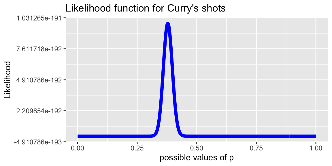
It looks like the most likely value of \(p\) is around 0.4.
We’ll write a function in R to calculate the value of \(p\) that maximizes the function.
7.3.6 Numerical Maximization
Lik.f <- function(nbasket,nmissed,nGrid){
    p <- seq(0, 1, length = nGrid)   # create nGrid values of p between 0 and 1
    lik <- p^{nbasket} * (1 - p)^{nmissed} # calculate value of lik at each p
    return(p[lik==max(lik)])             # find and return the value of p that maximizes the likelihood function
}## [1] 0.3785379The maximum likelihood estimate is \(\hat{p} = 0.3785\).
In fact, this is equal to 251/663. In this case, the MLE is consistent with our intuition.
7.3.7 MLE Using Calculus
We can also use calculus to find the value of \(p\) that maximizes the function \(\text{lik}(p)\).
In fact, it is usually easier to maximize the log of this function. We can do this since log is a non-decreasing function, ensuring that the value that maximizes \(\text{log}(\text{lik}(p))\) will also maximize \(\text{lik}(p)\).
\[ \begin{align*} \text{lik}(p) &= p^{251}(1-p)^{412} \\ \text{log}(\text{lik}(p)) &= 251\log(p)+412\log(1-p) \\ \frac{d}{dp} \log(\text{lik}(p)) &= \frac{251}{p} - \frac{412}{1-p} = 0 \end{align*} \]
and
\[ \frac{251}{p} = \frac{412}{1-p} \implies 251(1-p)=412p\implies p=\frac{251}{251+412}\approx0.3785 \]
7.3.8 Likelihood in a Logistic Regression Model
In a logistic regression model, we don’t try to estimate \(p\) directly, but rather to estimate \(\beta_0, \beta_1, \beta_p\), which are then used to calculate \(p\)
In our simple intercept only example,
\[p = \frac{e^{\beta_0}}{1+e^{\beta_0}}\]
and we need to estimate \(\beta_0\).
After removing constants, the new likelihood looks like:
\[ \begin{equation*} \begin{gathered} Lik(\beta_0) \propto \\ \left( \frac{e^{\beta_0}}{1+e^{\beta_0}}\right)^{251}\left(1- \frac{e^{\beta_0}}{1+e^{\beta_0}}\right)^{412} \end{gathered} \end{equation*} \]
7.3.9 Plot of Likelihood Function
library(ggplot2)
b=seq(-1,1,length=1001)
lik= (exp(b)/(1+exp(b)))^251*(1-(exp(b)/(1+exp(b))))^(412)       # likelihood of getting observed data
df <- data.frame(b,lik)
plot<- ggplot(data=df,aes(x=b, y=lik)) +
  geom_line(color="blue", size=2) +
  xlab("possible values of beta_0") + ylab("Likelihood") +
  labs(title="Likelihood function for Curry's shots")
plot + xlim(c(-1, 1))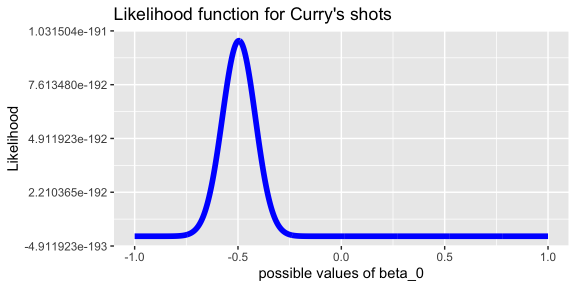
7.3.10 Numerical Maximization
Lik.f_logistic <- function(nbasket,nmissed,nGrid){
    b <- seq(-1, 1, length = nGrid)   # create values between -1 and 1 at which to evaluate the function
    lik <- (exp(b)/(1+exp(b)))^nbasket*(1-(exp(b)/(1+exp(b))))^nmissed  # calculate values at each b
    return(b[lik==max(lik)])    # find and return value of b that maximizes the function
}## [1] -0.4955496Our estimate is \(b_0 = -0.4955\).
From this we can calculate \[\hat{p} = \frac{e^{-0.4955}}{1+e^{-0.4955}}\approx0.3785\]
7.3.11 Comparison to R Output
Location <- c("Home", "Away")
Makes <- c(150, 101)
Misses <- c(247, 165)
Curry <- data.frame(Location, Makes, Misses)
head(Curry)
## Location Makes Misses
## 1 Home 150 247
## 2 Away 101 165##
## Call:
## glm(formula = cbind(Makes, Misses) ~ 1, family = binomial(link = "logit"),
## data = Curry)
##
## Coefficients:
## Estimate Std. Error z value Pr(>|z|)
## (Intercept) -0.49557 0.08007 -6.189 6.05e-10 ***
## ---
## Signif. codes: 0 '***' 0.001 '**' 0.01 '*' 0.05 '.' 0.1 ' ' 1
##
## (Dispersion parameter for binomial family taken to be 1)
##
## Null deviance: 0.0023559 on 1 degrees of freedom
## Residual deviance: 0.0023559 on 1 degrees of freedom
## AIC: 14.355
##
## Number of Fisher Scoring iterations: 2Note that the estimates differ in the 5th decimal place due to issues with numerical approximation. We could get a more precise approximation by increasing the number of points in our grid search.
We could maximize this function using calculus, which is more involved, but still doable in this case. Calculus-based methods typically do not work for more complicated likelihood methods involving more than one parameter, so we usually rely on numerical approximation methods.
7.3.12 Model for Home/Away
Now let’s build a model that allows Curry’s probability of making a shot to differ for away games, compared to home games.
Recall that Curry made 150 out of 397 shots at home and 101 out of 265 away.
Let \(p_H\) represent the probability of making a shot at home and \(p_A\) represent the probability of making a shot in an away game.
We can write the likelihood function as:
\[Lik(p_H, p_A) \propto p_H^{150}(1-p_H)^{247} p_A^{101}(1-p_A)^{165}\]
Our interest centers on estimating \(\hat{\beta_0}\) and \(\hat{\beta_1}\), not \(p_1\) or \(p_0\). So we replace \(p_1\) in the likelihood with an expression for \(p_1\) in terms of \(\beta_0\) and \(\beta_1\). Recall
\[p_i = \frac{e^{\beta_0+\beta_1\text{Home}}}{1+e^{\beta_0+\beta_1\text{Home}}}\]
After removing constants, the new likelihood looks like:
\[ \begin{equation*} \begin{gathered} Lik(\beta_0,\beta_1) \propto \\ \left( \frac{e^{\beta_0+\beta_1}}{1+e^{\beta_0+\beta_1}}\right)^{150}\left(1- \frac{e^{\beta_0+\beta_1}}{1+e^{\beta_0+\beta_1}}\right)^{247} \left(\frac{e^{\beta_0}}{1+e^{\beta_0}}\right)^{101}\left(1-\frac{e^{\beta_0}}{1+e^{\beta_0}}\right)^{165} \end{gathered} \end{equation*} \]
7.3.13 Numerical Optimization
Lik.f_logistic2 <- function(nbasketH,nmissedH,nbasketA,nmissedA,nGrid){
    b0 <- seq(-1, 1, length = nGrid)  # values of b0
    b1 <- seq(-1, 1, length=nGrid)  # values of b1
    B <- expand.grid(b0, b1)  # create all combinations of b0 and b1
    names(B) <- c("b0", "b1")  # give B the right names
    B <- B %>% mutate(Lik = (exp(b0+b1)/(1+exp(b0+b1)))^nbasketH*(1-(exp(b0+b1)/(1+exp(b0+b1))))^nmissedH*
                        (exp(b0)/(1+exp(b0)))^nbasketA*(1-(exp(b0)/(1+exp(b0))))^nmissedA) #evaluate function
    return(B[B$Lik==max(B$Lik),]) # find and return combination of b0 and b1 that maximize B.
}## b0 b1 Lik
## 496255 -0.4914915 -0.007007007 9.835399e-192Although we have worked with the likelihood function here, it is more common to work with the log of the likelihood function. Notice that the maximized log likelihood is very small, which can create numerical instability, though it doesn’t here.
7.3.14 Comparison to R Output
M <- glm(data = Curry, cbind(Makes, Misses) ~ Location , family = binomial(link="logit"))
summary(M)
##
## Call:
## glm(formula = cbind(Makes, Misses) ~ Location, family = binomial(link = "logit"),
## data = Curry)
##
## Coefficients:
## Estimate Std. Error z value Pr(>|z|)
## (Intercept) -0.490825 0.126339 -3.885 0.000102 ***
## LocationHome -0.007928 0.163330 -0.049 0.961286
## ---
## Signif. codes: 0 '***' 0.001 '**' 0.01 '*' 0.05 '.' 0.1 ' ' 1
##
## (Dispersion parameter for binomial family taken to be 1)
##
## Null deviance: 2.3559e-03 on 1 degrees of freedom
## Residual deviance: -4.2188e-15 on 0 degrees of freedom
## AIC: 16.353
##
## Number of Fisher Scoring iterations: 2The estimates are close to those that we obtained. We can make them closer by using a finer grid search.
7.3.15 Applications of Likelihood
Likelihood is at the heart of many of the model comparison tests we’ve worked with in this class.
Likelihood Ratio Tests
The ANOVA-type tests of reduced vs full models use likelihoods to calculate the improvement in fit, associated with adding additional variables to the model.
Our test statistic is
\[\begin{equation*} \begin{split} \textrm{LRT} &= 2[\max(\log(Lik(\textrm{larger model}))) - \max(\log(Lik(\textrm{reduced model})))] \\ &= 2\log\left(\frac{\max(Lik(\textrm{larger model}))}{\max(Lik(\textrm{reduced model}))} \right) \end{split} \end{equation*}\]
Statistical theory tells us that this statistic follows \(\chi^2\) distribution with the difference in number of parameters as its degrees of freedom.
In fact, it can be shown that the drop-in-deviance tests we’ve used for Poisson and logistic regression are special cases of this likelihood ratio test.
AIC and BIC
AIC and BIC are also calculated using the likelihood function.
\(\textrm{AIC} = -2 (\textrm{maximum log-likelihood }) + 2p\), where \(p\) represents the number of parameters in the fitted model. AIC stands for Akaike Information Criterion. Because smaller AICs imply better models, we can think of the second term as a penalty for model complexity—the more variables we use, the larger the AIC.
\(\textrm{BIC} = -2 (\textrm{maximum log-likelihood }) + p\log(n)\), where \(p\) is the number of parameters and \(n\) is the number of observations. BIC stands for Bayesian Information Criterion, also known as Schwarz’s Bayesian criterion (SBC).
7.3.16 Summary Maximum Likelihood Estimation
Maximum likelihood estimation is widely used to estimate parameters in many different kinds of statistical models
In LLSR, MLE and least-squares procedures yield the same estimates
Although they can be determined graphically, or using calculus in simple situations, MLE’s are usually approximated using numerical methods
It’s usually best, for reasons of numerical stability, to maximize the log of the likelihood function, rather than the likelihood function itself
In this section, we looked at a couple simple examples in logistic regression, but MLE’s are used in all of the models we’ve seen in this course (mixed effects, Poisson regression, etc.) and many more. It is the go-to technique for parameter estimation in classical frequentist statistics (which probably includes all statistics you’ve studied so far)
Maximum Likelihood estimation is taught in much more mathematical detail in STAT 445.
An alternative approach to Maximium Likelihood Estimation is Bayesian Estimation, which is taught in STAT 450
7.4 Zero-Inflated Poisson Model
7.4.1 Case Study: Weekend Drinking
Students in an introductory statistics class at a large university were asked:
“How many alcoholic drinks did you consume last weekend?”.
This survey was conducted on a dry campus where no alcohol is officially allowed, even among students of drinking age, so we expect that some portion of the respondents never drink. The purpose of this survey is to explore factors related to drinking behavior on a dry campus.
#Getting started-weekenddrinks
# File: weekendDrinks
drinks <- read.csv("https://raw.githubusercontent.com/proback/BeyondMLR/master/data/weekendDrinks.csv")
drinks <- drinks %>%
  mutate(off.campus=ifelse(dorm=="off campus",1,0),
         firstYear=dorm%in%c("kildahl","mohn","kittlesby")) %>% select(-c(dorm))
head(drinks)
## drinks sex off.campus firstYear
## 1 0 f 0 TRUE
## 2 5 f 0 FALSE
## 3 10 m 0 FALSE
## 4 0 f 0 FALSE
## 5 0 m 0 FALSE
## 6 3 f 0 FALSE7.4.2 Questions of Interest
- What proportion of students on this dry campus never drink?
- Do upper class students drink more than first years?
- What factors, such as off-campus living and sex, are related to whether students drink?
- Among those who do drink, to what extent is moving off campus associated with the number of drinks in a weekend?
- It is commonly assumed that males’ alcohol consumption is greater than females’; is this true on this campus?
7.4.3 Distribution of Number of Drinks
drinks %>% group_by(firstYear) %>% summarize(mean_drinks=mean(drinks),
                                             prop_zero = mean(drinks==0),
                                             n=n())
## # A tibble: 2 × 4
## firstYear mean_drinks prop_zero n
## <lgl> <dbl> <dbl> <int>
## 1 FALSE 2.41 0.407 59
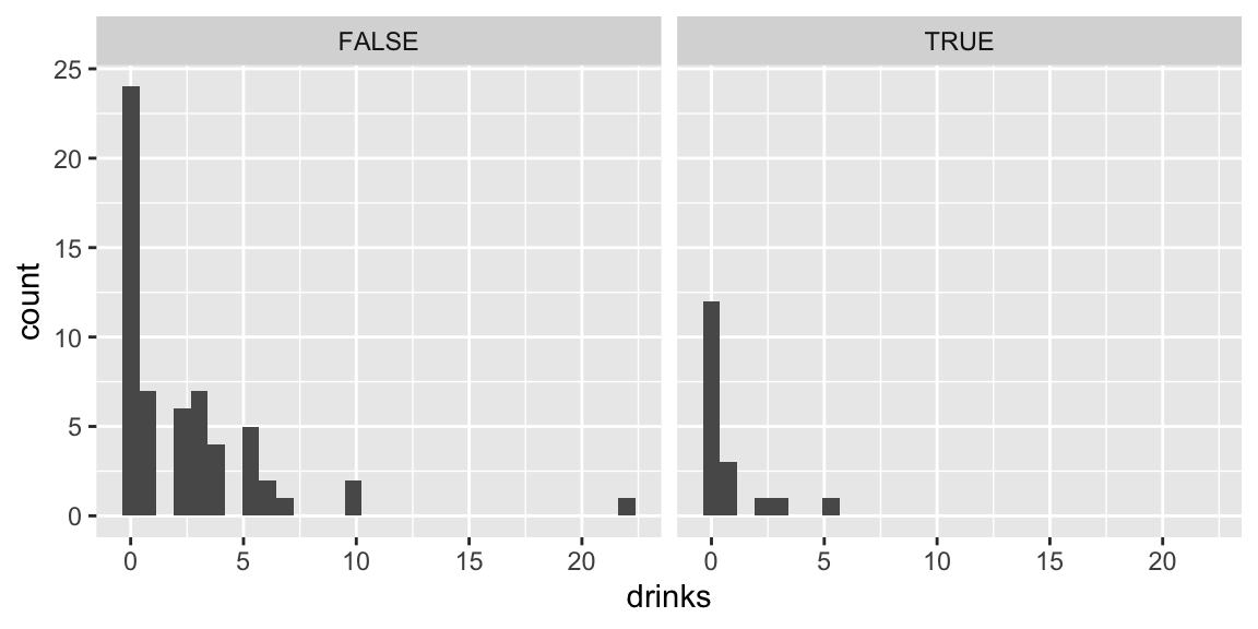
## 2 TRUE 0.722 0.667 187.4.4 Number of Drinks Comparisons
p1 <- ggplot(data = drinks) +
  geom_histogram(mapping = aes(x = drinks)) + facet_wrap(~firstYear, nrow=2) +
  ggtitle("Drinking by First Year Status")
p2 <- ggplot(data = drinks) +
  geom_histogram(mapping = aes(x = drinks)) + facet_wrap(~sex, nrow=2) +
  ggtitle("Drinks by Sex")
p3 <- ggplot(data = drinks) +
  geom_histogram(mapping = aes(x = drinks)) + facet_wrap(~off.campus, nrow=2) +
  ggtitle("Drinking by On/Off Campus")
grid.arrange(p1, p2, p3, nrow=1)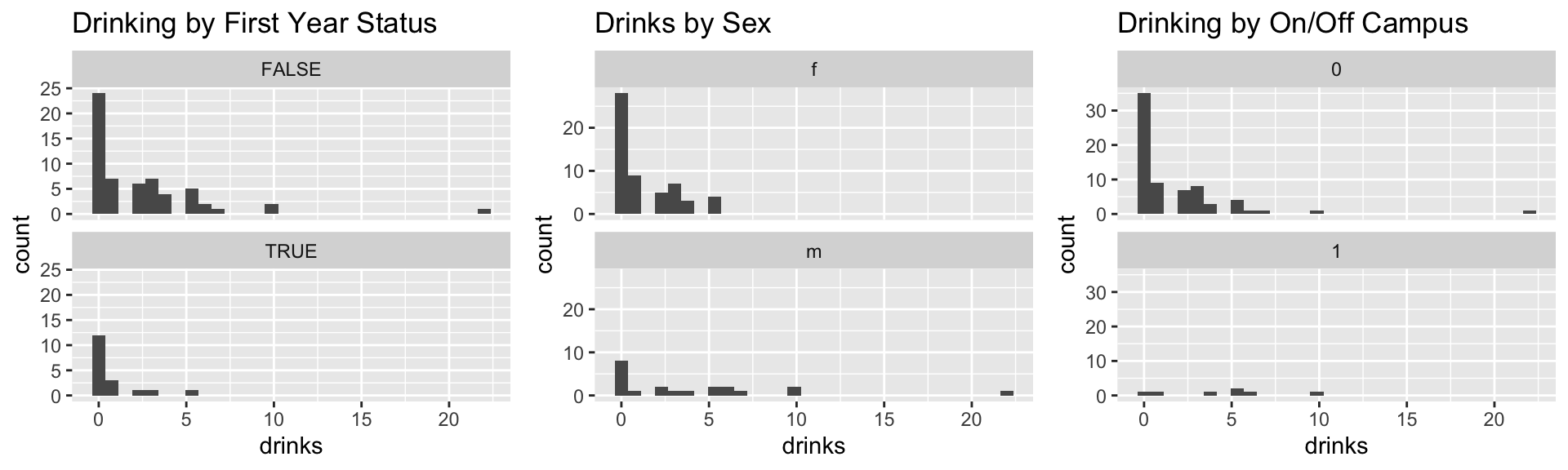
7.4.5 Proportion of Drinkers
Now, we compare proportions of students who reported drinking any drinks.
Drinks by First-Year Status:
p1 <- ggplot(data = drinks) +
  stat_count(mapping = aes(x = firstYear, fill=drinks>0), position="fill" ) +
  ggtitle("Drinking by First Year Status")
p2 <- ggplot(data = drinks) +
  stat_count(mapping = aes(x = sex, fill=drinks>0), position="fill" ) +
  ggtitle("Drinking by Sex")
p3 <- ggplot(data = drinks) +
  stat_count(mapping = aes(x = off.campus, fill=drinks>0), position="fill" ) +
  ggtitle("Drinking by On/Off Campus")
grid.arrange(p1, p2, p3, nrow=3)
7.4.6 Modeling Drinks
A Poisson distribution seems like a good choice for modeling drinks, since they are a count, and there is no fixed number of “attempts”, as in a binomial distribution.
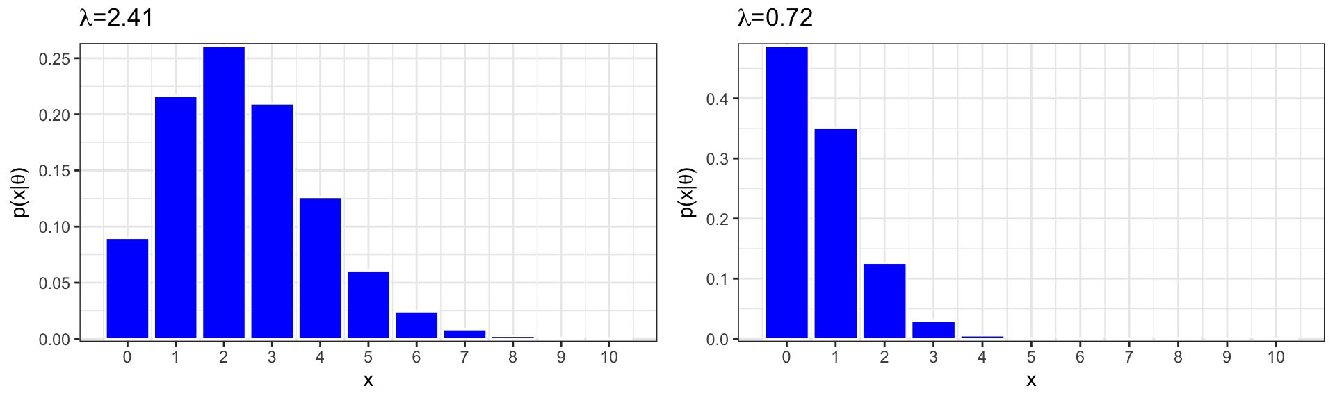
Expected Proportion of Zeros:
## [1] 0.08981529## [1] 0.4867523The proportion of zeros in our data is much higher than expected under a Poisson model with means equal to those observed in the data. (0.41 compared to 0.09 for upperclass students and 0.67, compared to 0.49 for first-years).
7.4.7 Explaining the Large Number of Zeros
The students who reported 0 drinks will fall into one of two categories:
- Students who do not drink at all.
- Students who do drink, but did not drink last weekend.
Our data consist of a mixture of responses from these two different populations.
Among students who do drink, it is reasonable to model the number of drinks consumed on a given weekend using a Poisson distribution
Among students who do not drink at all, there is no need to model the number of drinks in a given weekend, since we know it’s zero.
Ideally, we’d like to sort out the non-drinkers and drinkers when performing our analysis.
Answering these questions would be a simple matter if we knew who was and was not a drinker in our sample. Unfortunately, the non-drinkers did not identify themselves as such, so we will need to use the data available with a model that allows us to estimate the proportion of drinkers and non-drinkers.
7.4.8 Zero-Inflated Poisson Model
We’ll fit the model in two steps:
- Estimate the probability that a person drinks at all, given information contained in the explanatory variables.
- Model the number of drinks consumed in a given weekend, assuming the person does drink at all.
In step 1, we use logistic regression to estimate \(p\), the probability that the person does not drink at all.
In step 2, we use a Poisson regression to estimate \(\lambda\), the expected number of drinks a person consumes, assumping they drink at all.
7.4.9 Developing the Zero-Inflated Poisson Model
Let
\[ \begin{cases} 1 & \text{if student i drinks at all} \\ 0 & \text{if student i does not drink} \end{cases} \]
First, we model \(D_i\):
\[D_i\sim\text{Ber}(p_i) \]
and then \(Y_{i}\)
\[ \begin{cases} Y_i\sim\text{Pois}(\lambda_i) & \text{if } D_i=1 \\ Y_i=0 & \text{if } D_i=0 \end{cases} \]
The variable \(D_i\) is called a latent variable. It is a variable that is relevant to the process we are interested in studying, but is not directly measured or reported in our data.
The Zero-Inflated Poisson is an example of a mixture model, as the response variable is modeled using a mixture of Bernoulli and Poisson distributions.
Let \(p_i\) represent \(P(D_i=0)\), the probability that person person does not drink.
7.4.10 Deriving the ZIP PMF
We derive the probability mass function for the Poisson model by considering the two different ways we can observe count \(y\).
\[ \begin{aligned} P(Y=0) &= P(\text{Person Doesn't Drink at All}) + P(\text{Person drinks and didn't drink last week})\\ & = P(\text{Person Doesn't Drink at All}) + P(\text{0 drinks in a given weekend given person drinks})P(\text{Person drinks}) \\ & = P(D_i=0) + P(Y_i=0|D_i=1)P(D_i=1) \\ & = p_i + \frac{\lambda_i^0e^{-\lambda_i}}{0!}(1-p) \\ & = p_i + e^{-\lambda_i}(1-p_i) \end{aligned} \]
For \(y\neq 0\),
\[ \begin{aligned} P(Y=y) &= P(\text{Person drinks and drinks y drinks in a weekend})\\ & = P(\text{y drinks in a given weekend given person drinks})P(\text{Person drinks}) \\ & = P(Y_i=y|D_i=1)P(D_i=1) \\ & = \frac{\lambda_i^ye^{-\lambda_i}}{y!}(1-p) \end{aligned} \]
Putting these together, we get the ZIP probability mass function:
\[ P(Y=y) = \begin{cases} p_i + e^{-\lambda_i}(1-p_i) & \text{if } y=0 \\ \frac{\lambda_i^ye^{-\lambda_i}}{y!}(1-p_i) & \text{if } y>0 \end{cases} \]
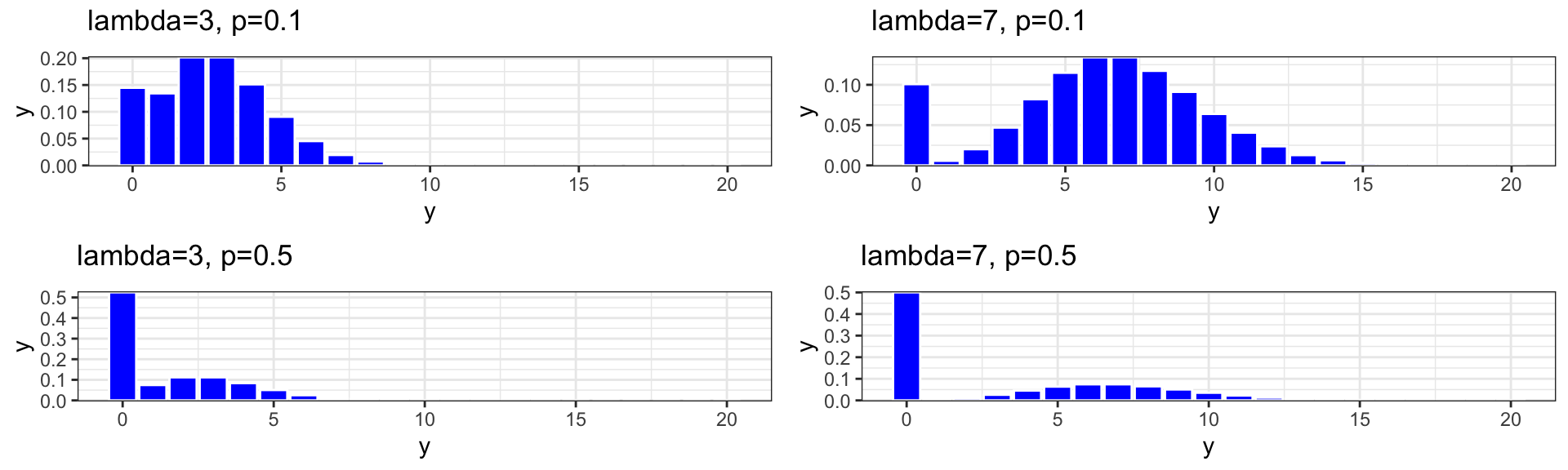
7.4.12 ZIP Model
We assume
\[ Y_i \sim\text{ZIP}(p_i, \lambda_i) \]
\(p_i\) represents the probability that student \(i\) drinks at all.
\(\lambda_i\) represents the average number of drinks student \(i\) consumes in a weekend, assuming they do drink at all.
We want to estimate \(p_i\) and \(\lambda_i\), using information contained in the explanatory variables.
We can use different explanatory variables to estimate \(p_i\) and \(\lambda_i\).
Let \(Z_{1}, Z_2, \ldots, Z_p'\) be the explanatory variables used to estimate \(p\), and \(X_1, X_2, \ldots, X_p\) be the explanatory variables used to estimate \(\lambda\)
We link \(p_i\) and \(\lambda_i\) to a linear combination of the explanatory variables, using the link functions:
\[ log(\lambda_i) = \beta_0+\beta_1X_{i1}+ \ldots +\beta_pX_{ip}, \]
\[ log\left(\frac{p_i}{1-p_i}\right) = \alpha_0+\alpha_1Z_{i1}+ \ldots +\alpha_pZ_{ip'}, \]
We obtain estimates of \(\beta_0, \ldots{\beta_p}\) and \(\alpha_0, \ldots, \alpha_p\), and from these obtain maximum likelihood etimates for \(p_i\) and \(\lambda_i\).
7.5 Model for Drinks Data
7.5.1 ZIP for Drinks Data
A zero-inflated Poisson regression model to take non-drinkers into account consists of two parts:
- One part models the association, among drinkers, between number of drinks and the predictors of sex and off-campus residence.
- The other part uses a predictor for first-year status to obtain an estimate of the proportion of non-drinkers based on the reported zeros.
The form for each part of the model follows. The first part looks like an ordinary Poisson regression model:
\[ log(\lambda_i)=\beta_0+\beta_1\textrm{off.campus}_i+ \beta_2\textrm{sex}_i \] where \(\lambda\) is the mean number of drinks in a weekend among those who drink. The second part has the form
\[ logit(p_i)=\alpha_0+\alpha_1\textrm{firstYear}_i \] where \(\alpha\) is the probability of being in the non-drinkers group and \(logit(p_i) = log( p_i/(1-p_i))\).
7.5.2 ZIP Model in R
We will use the R function zeroinfl from the package pscl to fit a ZIP model. The terms before the | are used to model expected number of drinks, assuming the person really does drink at all.
The terms after the | are used to estimate the probability that the person drinks at all.
Call:
zeroinfl(formula = drinks ~ off.campus + sex | firstYear, data = drinks)

Pearson residuals:
    Min      1Q  Median      3Q     Max
-1.1118 -0.8858 -0.5290  0.6367  5.2996

Count model coefficients (poisson with log link):
            Estimate Std. Error z value Pr(>|z|)
(Intercept)   0.7543     0.1440   5.238 1.62e-07 ***
off.campus    0.4159     0.2059   2.020   0.0433 *
sexm          1.0209     0.1752   5.827 5.63e-09 ***

Zero-inflation model coefficients (binomial with logit link):
              Estimate Std. Error z value Pr(>|z|)
(Intercept)    -0.6036     0.3114  -1.938   0.0526 .
firstYearTRUE   1.1364     0.6095   1.864   0.0623 .
---
Signif. codes:  0 '***' 0.001 '**' 0.01 '*' 0.05 '.' 0.1 ' ' 1

Number of iterations in BFGS optimization: 8
Log-likelihood: -140.8 on 5 Df## count_(Intercept) count_off.campus count_sexm zero_(Intercept)
## 2.1260699 1.5157953 2.7756910 0.5468311
## zero_firstYearTRUE
## 3.1154950Interpretations
For those who drink, the average number of drinks for males is \(e^{1.0209}\) or 2.76 times the number for females (Z = 5.827, p < 0.001) given that you are comparing people who live in comparable settings (on or off campus)
Among drinkers, the mean number of drinks for students living off campus is \(e^{0.4159}=1.52\) times that of students living on campus for those of the same sex (Z = 2.021, p = 0.0433).
The odds that a first-year student is a non-drinker are 3.12 times the odds that an upper-class student is a non-drinker.
The estimated probability that a first-year student is a non-drinker is
\[ \frac{e^{0.533}}{1+e^{0.533}} = 0.630 \]
or 63.0%, while for non-first-year students, the estimated probability of being a non-drinker is 0.354.
7.5.3 Residual Plot
Fitted values (\(\hat{y}\)) and residuals (\(y-\hat{y}\)) can be computed for zero-inflation models and plotted. Figure 7.1 reveals that one observation appears to be extreme (Y=22 drinks during the past weekend). Is this a legitimate observation or was there a transcribing error? Without the original respondents, we cannot settle this question. It might be worthwhile to get a sense of how influential this extreme observation is by removing Y=22 and refitting the model.
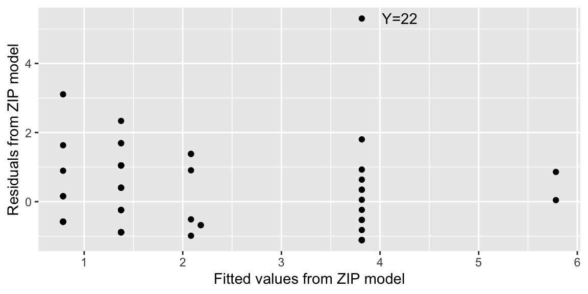
Figure 7.1: Residuals by fitted counts for ZIP model.
7.5.4 Limitations
There are several concerns and limitations we should think about related to this study.
What time period constitutes the “weekend”?
What constitutes a drink—a bottle of beer?
How many drinks will a respondent report for a bottle of wine?
There is also an issue related to confidentiality. If the data is collected in class, will the teacher be able to identify the respondent? Will respondents worry that a particular response will affect their grade in the class or lead to repercussions on a dry campus?
In addition to these concerns, there are a number of other limitations that should be noted. Following the concern of whether this data represents a random sample of any population (it doesn’t), we also must be concerned with the size of this data set (77). ZIP models are not appropriate for small samples and this data set is not impressively large.
7.5.5 Final Thoughts on Zero-Inflated Models
At times, a mixture of zeros occurs naturally. It may not come about because of neglecting to ask a critical question on a survey, but the information about the subpopulation may simply not be ascertainable. For example, visitors from a state park were asked as they departed how many fish they caught, but those who report 0 could be either non-fishers or fishers who had bad luck. These kinds of circumstances occur often enough that ZIP models are becoming increasingly common.
Actually, applications which extend beyond ordinary Poisson regression applications—ZIPs and other Poisson modeling approaches such as hurdle models and quasi-Poisson applications—are becoming increasingly common. So it is worth taking a look at these variations of Poisson regression models. Here we have only skimmed the surface of zero-inflated models, but we want you to be aware of models of this type. ZIP models demonstrate that modeling can be flexible and creative—a theme we hope you will see throughout this book.
7.6 Practice Problems
In the professional National Basketball Association (NBA), each team plays 82 games in a season. We have data on the season that ended in 2018. In basketball, teams can attempt either 2-point shots, or 3-point shots, which are taken further from the basket. We’ll investigate whether taking more 3-point shots improves or hurts a team’s chances of winning a game. We model the number of wins for each of the league’s 30 teams, using percentage of shots taken that were 3 point shots as an explanatory variable.
NBA <- read.csv("https://raw.githubusercontent.com/proback/BeyondMLR/master/data/NBA1718team.csv")
NBA <- NBA %>% mutate(PCT3P = attempts_3P/(attempts_2P+attempts_3P)*100)
The first 5 rows of the data are shown below.
##   TEAM Win Loss    PCT3P
## 1  ATL  24   58 36.26515
## 2  BKN  28   54 41.10205
## 3  BOS  55   27 35.72760
## 4  CHA  36   46 31.42415
## 5  CHI  27   55 34.98970
Output for a binomial logistic regression model is shown below.
##
## Call:
## glm(formula = cbind(Win, Loss) ~ PCT3P, family = binomial(link = "logit"),
##     data = NBA)
##
## Coefficients:
##              Estimate Std. Error z value Pr(>|z|)
## (Intercept) -1.118837   0.298581  -3.747 0.000179 ***
## PCT3P        0.033202   0.008785   3.780 0.000157 ***
## ---
## Signif. codes:  0 '***' 0.001 '**' 0.01 '*' 0.05 '.' 0.1 ' ' 1
##
## (Dispersion parameter for binomial family taken to be 1)
##
##     Null deviance: 217.97  on 29  degrees of freedom
## Residual deviance: 203.42  on 28  degrees of freedom
## AIC: 350.54
##
## Number of Fisher Scoring iterations: 3
40. State the assumptions associated with a binomial logistic regression model and determine whether the assumptions are satisfied.
Explain why a binomial logistic model is more appropriate for these data than an LLSR model or a Poisson regression model.
Explain how we could check the constant linearity assumption in the binomial logistic model. Write out the coordinates of at least two of the points you would plot.
Explain how you would check the variance assumption with the binomial logistic plot. Why might this be challenging?
41. Calculate probabilities and odds and expected changes associated with fixed effects in a binomial logistic regression model.
Calculate the estimated probability of a team that shoots 35 percent of its shots as 3-pointers winning a game.
If one team is estimated to have a 0.5 probability of winning, and another team’s percentage of three point shots attempted is 4 percentage points higher, what is the second team’s estimated probability of winning?
42. Interpret fixed effect coefficients in a binomial logistic regression model.
Interpret both estimates in the coefficients table.
44. Interpret fixed effect coefficients in a Zero-Inflated Poisson model.
Using a sample of 5,190 people, taken by the Australian Health Service 1977-78, we model the number of times a person visited the doctor during a 2 week span. Possible explanatory variables include age, and whether or not the person had free health insurance provided through a government program for low-income residents. The variable is called freepoor.
| visits | age | freepoor |
|---|---|---|
| 1 | 19 | no |
| 1 | 19 | no |
| 1 | 19 | no |
| 1 | 19 | no |
| 1 | 19 | no |
| 1 | 19 | no |
We use a zero-inflated model to model number of doctor visits, using age and freepoor as explanatory variables.
library(pscl)
M_ZIP <- zeroinfl(visits ~ age + freepoor | age + freepoor,
                   data = DoctorVisits)
summary(M_ZIP)
Call:
zeroinfl(formula = visits ~ age + freepoor | age + freepoor, data = DoctorVisits)

Pearson residuals:
    Min      1Q  Median      3Q     Max
-0.5597 -0.4803 -0.3737 -0.3640 13.6623

Count model coefficients (poisson with log link):
             Estimate Std. Error z value Pr(>|z|)
(Intercept) -0.320817   0.106466  -3.013  0.00258 **
age          0.003437   0.001971   1.744  0.08124 .
freepooryes  0.461781   0.251507   1.836  0.06635 .

Zero-inflation model coefficients (binomial with logit link):
             Estimate Std. Error z value Pr(>|z|)
(Intercept)  1.357795   0.142682   9.516  < 2e-16 ***
age         -0.018593   0.002914  -6.379 1.78e-10 ***
freepooryes  1.058227   0.294661   3.591 0.000329 ***
---
Signif. codes:  0 '***' 0.001 '**' 0.01 '*' 0.05 '.' 0.1 ' ' 1

Number of iterations in BFGS optimization: 14
Log-likelihood: -3646 on 6 Df
Interpret the age coefficient for both parts of the model.
Interpret the freepooryes coefficient for both parts of the model.