Chapter 5 Data with Three or More Levels
Chapter 5 Learning Outcomes
Identify the levels of a three-level experiment and the observational units and variables at each level.
Interpret fixed and random effects and associated parameter estimates in models with three or more levels.
Write equations for linear mixed effects models in mathematical notation, including assumptions about distributions of random effects and error terms for models with three or more levels.
These notes accompany Chapter 10 in Beyond Multiple Linear Regression by Roback and Legler.
# Packages required for Chapter 10
library(MASS)
library(gridExtra)
library(mnormt)
library(lme4)
library(lmerTest)
library(knitr)
library(kableExtra)
library(tidyverse)
library(Hmisc)
library(nlme)
5.1 Three-Level Plants Experiment
5.1.1 Experimental Design
Researchers are interested in comparing heights of plants of two different genotypes (A and B), with two different fertilizers (A and B), and also in assessing whether being close to window affects growth. Scientists obtained four trays and placed four pots in each tray. Two of the trays were placed close to windows and the other two were placed away from windows. Within each tray, two of the pots received fertilizer A and two received fertilizer B. Two plants of each phenotype were then planted in each plot. After 4 weeks, researchers recorded the height of each plant.
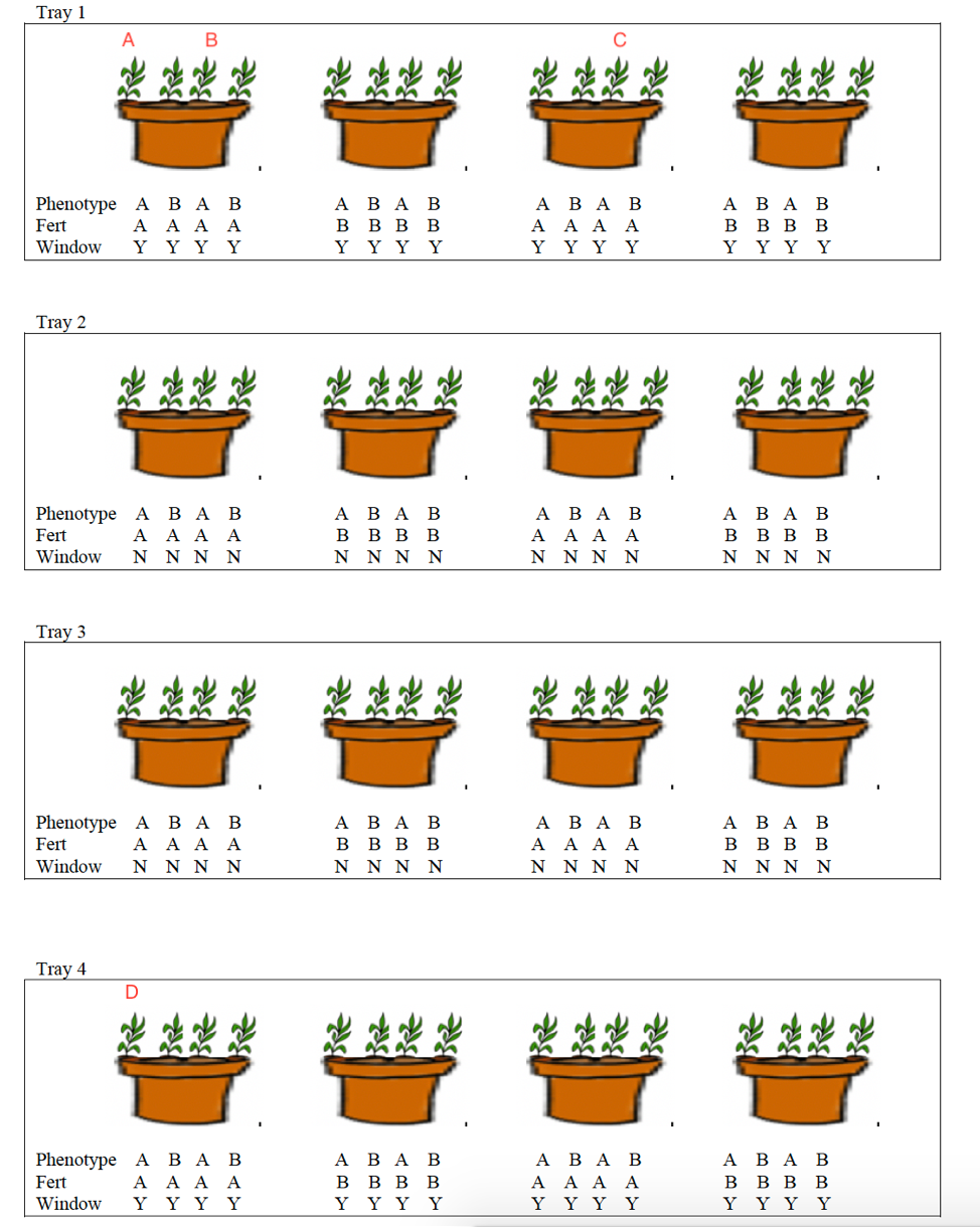
Figure 5.1: Potted Plant Experimental Design
5.1.2 The Data
The first 20 rows of the dataset are shown below.
##    plantid tray pot window fertA phenoA height
## 1        1    1   1      1     1      1   5.59
## 2        2    1   1      1     1      0   5.33
## 3        3    1   1      1     1      1   5.70
## 4        4    1   1      1     1      0   5.77
## 5        5    1   2      1     0      1   2.93
## 6        6    1   2      1     0      0   1.79
## 7        7    1   2      1     0      1   2.57
## 8        8    1   2      1     0      0   2.12
## 9        9    1   3      1     1      1   4.86
## 10      10    1   3      1     1      0   2.13
## 11      11    1   3      1     1      1   3.24
## 12      12    1   3      1     1      0   2.10
## 13      13    1   4      1     0      1   1.10
## 14      14    1   4      1     0      0   2.35
## 15      15    1   4      1     0      1   1.79
## 16      16    1   4      1     0      0   4.88
## 17      17    2   5      0     1      1   1.51
## 18      18    2   5      0     1      0   3.71
## 19      19    2   5      0     1      1   2.30
## 20      20    2   5      0     1      0   2.30
5.1.3 Questions
- Between plants B, C, and D, which would you expect to be most highly correlated with plant A? Which would you expect to be least highly correlated with plant A?
- What are the observational units at each level? What are the treatments or variables?
5.1.4 Three Level Model
Let \(Y_{ijk}\) represent the height of plant \(k\) in pot \(j\) in tray \(i\). A possible model is:
\[ \begin{align*} Y_{ijk} & = [\alpha_{0}+\alpha_{1}\textrm{Window}_{i}+\beta_{0}\textrm{FertA}_{ij}+\gamma_{0}\textrm{PhenoA}_{ijk}] \\ & \textrm{} + [t_{i}+ p_{ij} + \epsilon_{ijk}], \end{align*} \]
where \(t_i\sim N(0, \sigma^2_t)\), \(p_{ij}\sim N(0, \sigma^2_p)\), and \(\epsilon_{ijk}\sim N(0, \sigma^2)\)
This model includes fixed effects for window, fertilizer, and phenotype, and random effects for tray and pot. We assume there are no interactions between the fixed effects.
The model includes 3 random effects:
- \(t_i\) - deviations in average plant heights between trays, after accounting for the three fixed effects.
- \(p_{ij}\) - deviations in average plant height between pots in the same tray, after accounting for the three fixed effects.
- \(\epsilon_{ijk}\) - deviations between individual plants in the same tray and pot after accounting for the three fixed effects.
The model does not include any random slope effects. This means we are assuming the effect of phenotype is the same in each pot, and the effect of fertilizer is the same in each tray.
5.1.5 R Implementation of Three Level Model
## Linear mixed model fit by REML. t-tests use Satterthwaite's method [
## lmerModLmerTest]
## Formula: height ~ window + fertA + phenoA + (1 | pot) + (1 | tray)
##    Data: plants
##
## REML criterion at convergence: 201.6
##
## Scaled residuals:
##      Min       1Q   Median       3Q      Max
## -2.35859 -0.61695 -0.06346  0.56342  2.27449
##
## Random effects:
##  Groups   Name        Variance Std.Dev.
##  pot      (Intercept) 0.4784   0.6917
##  tray     (Intercept) 0.1336   0.3655
##  Residual             1.0775   1.0380
## Number of obs: 64, groups:  pot, 16; tray, 4
##
## Fixed effects:
##             Estimate Std. Error      df t value Pr(>|t|)
## (Intercept)   2.1178     0.4731  3.8400   4.476   0.0121 *
## window        1.1416     0.5662  2.0000   2.016   0.1813
## fertA         0.7528     0.4324 11.0000   1.741   0.1095
## phenoA        0.5997     0.2595 47.0000   2.311   0.0253 *
## ---
## Signif. codes:  0 '***' 0.001 '**' 0.01 '*' 0.05 '.' 0.1 ' ' 1
##
## Correlation of Fixed Effects:
##        (Intr) window fertA
## window -0.598
## fertA  -0.457  0.000
## phenoA -0.274 0.000 0.000\(\hat{\sigma}_p=0.6917\), \(\hat{\sigma}_t=0.3655\), \(\hat{\sigma}=1.0380\).
After accounting for phenotype, fertilizer, and window, the greatest amount of remaining variability occurs between individual plants in the same pot, followed by average heights among pots in the same tray, followed by average heights between trays.
5.1.6 Inappropriate LLSR Model
We compare this to an inappropriately fit LLSR model.
##
## Call:
## lm(formula = height ~ window + fertA + phenoA, data = plants)
##
## Residuals:
##     Min      1Q  Median      3Q     Max
## -2.7591 -0.9762  0.2752  0.8677  2.1381
##
## Coefficients:
##             Estimate Std. Error t value      Pr(>|t|)
## (Intercept)   2.1178     0.3126   6.775 0.00000000604 ***
## window        1.1416     0.3126   3.652      0.000548 ***
## fertA         0.7528     0.3126   2.408      0.019115 *
## phenoA        0.5997     0.3126   1.918      0.059814 .
## ---
## Signif. codes:  0 '***' 0.001 '**' 0.01 '*' 0.05 '.' 0.1 ' ' 1
##
## Residual standard error: 1.25 on 60 degrees of freedom
## Multiple R-squared:  0.2755, Adjusted R-squared:  0.2393
## F-statistic: 7.606 on 3 and 60 DF,  p-value: 0.0002161
the LLSR model inappropriately assumes we have 64 independent observations
Since the phenotype variable pertains to the 64 individual plants, the “effective” sample size for inference about phenotype is still 64. Since we are able to randomly assign phenotypes within pots, the multilevel model accounts for variability associated with pot and tray, taking \(\sigma^2_t\) and \(\sigma^2_p\) out of the calculation of \(\sigma^2\) in the LSSR model, resulting in a smaller standard error associated with phenotype.
Since fertilizer was assigned to pots, rather than plants, the “effective” sample size is 16. This smaller sample size leads to higher standard error associated with the effect of fertilizer.
Since window was assigned to trays, the “effective” sample size is 4, resulting in the highest standard errors being associated with trays.
5.2 Three-Level Model with Random Slopes
5.2.1 Random Slope for PhenoA
We could allow for the possibility that the effect of phenotype is different in different pots, by adding a random slope effect for phenotype.
\[ \begin{align*} Y_{ijk} & = [\alpha_{0}+\alpha_{1}\textrm{Window}_{i}+\beta_{0}\textrm{FertA}_{ij}+\gamma_{0}\textrm{PhenoA}_{ijk}] \\ & \textrm{} + [t_i + p_{ij} + q_{ij}\textrm{PhenoA}_{ijk} + \epsilon_{ijk}], \end{align*} \]
where \(t_i\sim N(0, \sigma^2_t)\), and \(\epsilon_{ijk}\sim N(0, \sigma^2)\)
\[ \left[ \begin{array}{c} p_{ij} \\q_{ij} \end{array} \right] \sim N \left( \left[ \begin{array}{c} 0 \\ 0 \end{array} \right], \left[ \begin{array}{cc} \sigma_{p}^{2} & \rho_{pq}\sigma_{p}\sigma_q \\ \rho_{pq}\sigma_{p}\sigma_q & \sigma_{q}^{2} \end{array} \right] \right) \]
We assume random error terms on different levels are independent of each other. That is, \(t_i\) is independent of \(p_{ij}\) and \(q_{ij}\), and all of these are independent of \(\epsilon_{ijk}\).
5.2.2 R Output for Random Slope for PhenoA
## Linear mixed model fit by REML. t-tests use Satterthwaite's method [
## lmerModLmerTest]
## Formula: height ~ window + fertA + phenoA + (phenoA | pot) + (1 | tray)
##    Data: plants
##
## REML criterion at convergence: 200.2
##
## Scaled residuals:
##      Min       1Q   Median       3Q      Max
## -2.16998 -0.65343 -0.06843  0.67860  1.97927
##
## Random effects:
##  Groups   Name        Variance Std.Dev. Corr
##  pot      (Intercept) 0.6371   0.7982
##           phenoA      0.5754   0.7586   -0.42
##  tray     (Intercept) 0.1221   0.3494
##  Residual             0.8938   0.9454
## Number of obs: 64, groups:  pot, 16; tray, 4
##
## Fixed effects:
##             Estimate Std. Error      df t value Pr(>|t|)
## (Intercept)   2.1268     0.4719  3.5371   4.506   0.0142 *
## window        1.1380     0.5567  1.8497   2.044   0.1879
## fertA         0.7384     0.4334 10.8398   1.704   0.1169
## phenoA        0.5997     0.3030 15.0002   1.979   0.0665 .
## ---
## Signif. codes:  0 '***' 0.001 '**' 0.01 '*' 0.05 '.' 0.1 ' ' 1
##
## Correlation of Fixed Effects:
##        (Intr) window fertA
## window -0.590
## fertA  -0.459  0.000
## phenoA -0.305  0.000  0.000
The negative estimate of correlation \(\rho_{pq}\) indicates that differences between phenotypes are smaller in pots when plants of phenotype B are taller.
5.2.3 Random Slope for Fert
What if we want to allow for the possibility that the effects of fertilizers varies between trays?
The R code for such a model is shown below.
How would we write this model mathematically? Include any distributional assumptions about the random effects and error terms.
5.2.4 R Output for Random Slope for Fert
## Linear mixed model fit by REML. t-tests use Satterthwaite's method [
## lmerModLmerTest]
## Formula: height ~ window + fertA + phenoA + (1 | pot) + (fertA | tray)
##    Data: plants
##
## REML criterion at convergence: 201.1
##
## Scaled residuals:
##      Min       1Q   Median       3Q      Max
## -2.34479 -0.62506 -0.01316  0.55385  2.38204
##
## Random effects:
##  Groups   Name        Variance Std.Dev. Corr
##  pot      (Intercept) 0.3905   0.6249
##  tray     (Intercept) 0.4759   0.6899
##           fertA       0.2731   0.5226   -1.00
##  Residual             1.0775   1.0380
## Number of obs: 64, groups:  pot, 16; tray, 4
##
## Fixed effects:
##             Estimate Std. Error      df t value Pr(>|t|)
## (Intercept)   1.9829     0.5404  3.0907   3.669   0.0333 *
## window        1.4115     0.5430  2.7821   2.599   0.0869 .
## fertA         0.7528     0.4830  3.8691   1.559   0.1964
## phenoA        0.5997     0.2595 47.0000   2.311   0.0253 *
## ---
## Signif. codes:  0 '***' 0.001 '**' 0.01 '*' 0.05 '.' 0.1 ' ' 1
##
## Correlation of Fixed Effects:
##        (Intr) window fertA
## window -0.502
## fertA  -0.661  0.000
## phenoA -0.240  0.000  0.000
## optimizer (nloptwrap) convergence code: 0 (OK)
## boundary (singular) fit: see help('isSingular')
5.2.5 Boundary Constraints
Recall that \(-1\leq\rho\leq1\), where \(\rho\) represents the correlation between random effects at the same level. When \(\hat{\rho}=\pm1\), this indicates that the maximimum likelihood estimates are occuring along a boundary of this range, usually making them unreliable.
In these situations, we should not draw conclusions basde on \(\rho\) and should consider dropping this random effect from the model.
We could also add interaction or nonlinear terms for fixed effects if we had reason to do so.
5.3 Longitudinal Component to Plants Data
5.3.1 Repeated Measures over Time
Now suppose that in addition to this first measurement, the heights of the same plants were recorded again once per week for 4 weeks.
##    plantid time tray pot window fertA phenoA   height
## 1        1    1    1   1      1     1      1 5.593006
## 2        1    2    1   1      1     1      1 6.588438
## 3        1    3    1   1      1     1      1 7.483192
## 4        1    4    1   1      1     1      1 8.889305
## 5        2    1    1   1      1     1      0 5.330448
## 6        2    2    1   1      1     1      0 6.350843
## 7        2    3    1   1      1     1      0 7.380016
## 8        2    4    1   1      1     1      0 8.442597
## 9        3    1    1   1      1     1      1 5.700156
## 10       3    2    1   1      1     1      1 6.549357
## 11       3    3    1   1      1     1      1 7.742034
## 12       3    4    1   1      1     1      1 8.892204
## 13       4    1    1   1      1     1      0 5.770243
## 14       4    2    1   1      1     1      0 6.550047
## 15       4    3    1   1      1     1      0 7.632318
## 16       4    4    1   1      1     1      0 8.796274
## 17       5    1    1   2      1     0      1 2.925716
## 18       5    2    1   2      1     0      1 3.626215
## 19       5    3    1   2      1     0      1 4.687552
## 20       5    4    1   2      1     0      1 5.433369
5.3.2 Levels and Variables
Now, this is a 4-level dataset.
| Level | Observational Unit | Treatment or Variable |
|---|---|---|
| Level 1 | time points | time |
| Level 2 | plants | phenotype |
| Level 3 | pots | fertilizer |
| Level 4 | trays | window |
5.3.3 Model for Longitudinal Plants Study
Let \(Y_{ijkl}\) represent the height of plant \(k\) in pot \(j\) in tray \(i\) at time \(l\). A possible model is:
\[ \begin{align*} Y_{ijkl} & = [\alpha_{0}+\alpha_{1}\textrm{Window}_{i}+\beta_{0}\textrm{FertA}_{ij}+\gamma_{0}\textrm{PhenoA}_{ijk} + \delta_{0}\textrm{Time}_{ijkl}] \\ & \textrm{} + [t_{i}+ p_{ij} + f_{ijk} + \epsilon_{ijkl}], \end{align*} \]
where \(t_i\sim N(0, \sigma^2_t)\), \(p_{ij}\sim N(0, \sigma^2_p)\), \(f_{ijk}\sim N(0, \sigma^2_f)\),and \(\epsilon_{ijkl}\sim N(0, \sigma^2)\)
This model involves random intercepts for each tray(\(t_i\)), pot(\(p_{ij}\)), plant (\(f_{ijk}\)), in addition to a random error term \(\epsilon{ijkl}\) capturing random differences between measurements on the same plant over time.
In addition to the assumptions of model 1, it assumes each plant grows at the same rate over time, after accounting for the fixed effects in the model.
5.3.4 R Output for Longitudinal Model
M5 <- lmer(data=plants, height ~ window + fertA + phenoA + time + (1|tray) + (1|pot) + (1|plantid))
summary(M5)
## Linear mixed model fit by REML. t-tests use Satterthwaite's method [
## lmerModLmerTest]
## Formula: height ~ window + fertA + phenoA + time + (1 | tray) + (1 | pot) +
## (1 | plantid)
## Data: plants
##
## REML criterion at convergence: 362.3
##
## Scaled residuals:
## Min 1Q Median 3Q Max
## -2.81419 -0.56459 -0.00598 0.56245 2.67726
##
## Random effects:
## Groups Name Variance Std.Dev.
## plantid (Intercept) 1.10406 1.0507
## pot (Intercept) 0.77702 0.8815
## tray (Intercept) 0.07314 0.2705
## Residual 0.08029 0.2834
## Number of obs: 256, groups: plantid, 64; pot, 16; tray, 4
##
## Fixed effects:
## Estimate Std. Error df t value Pr(>|t|)
## (Intercept) 1.21075 0.50407 4.40523 2.402 0.0683 .
## window 1.47080 0.58108 2.00001 2.531 0.1270
## fertA 0.90342 0.51431 11.00003 1.757 0.1068
## phenoA 0.58651 0.26506 47.00038 2.213 0.0318 *
## time 0.66370 0.01584 190.99990 41.899 <0.0000000000000002 ***
## ---
## Signif. codes: 0 '***' 0.001 '**' 0.01 '*' 0.05 '.' 0.1 ' ' 1
##
## Correlation of Fixed Effects:
## (Intr) window fertA phenoA
## window -0.576
## fertA -0.510 0.000
## phenoA -0.263 0.000 0.000
## time -0.079 0.000 0.000 0.000We see that after accounting for time, phenotype, fertilizer, and window location, there is more variability between average heights of different plants in the same pot (\(\sigma_f=1.05\)), and in average heights in different pots in the same tray (\(\sigma_p=0.88\)), than between average heights in different trays(\(\sigma_t=0.27\)), or between heights of the same plant at different times(\(\sigma=0.28\)).
There is evidence that plants grow over time, and evidence of differences between the phenotypes.
5.4 Four-Level Longitudinal Model with Random Slopes
5.4.1 Random Slope for Time
We could add a random error term associated with the slope on time, to allow for the possibility that individual plants grow at different rates, even after accounting for the fixed effects in the model
\[ \begin{align*} Y_{ijkl} & = [\alpha_{0}+\alpha_{1}\textrm{Window}_{i}+\beta_{0}\textrm{FertA}_{ij}+\gamma_{0}\textrm{PhenoA}_{ijk} + \delta_{0}\textrm{Time}_{ijkl}] \\ & \textrm{} + [t_{i}+ p_{ij} + f_{ijk} + g_{ijk}\textrm{Time}_{ijkl} + \epsilon_{ijkl}], \end{align*} \]
where \(t_i\sim N(0, \sigma^2_t)\), \(p_{ij}\sim N(0, \sigma^2_p)\), \(\epsilon_{ijkl}\sim N(0, \sigma^2)\), and
\[ \begin{equation*} \left[ \begin{array}{c} f_{ijk} \\g_{ijk} \end{array} \right] \sim N \left( \left[ \begin{array}{c} 0 \\ 0 \end{array} \right], \left[ \begin{array}{cc} \sigma_{f}^{2} & \rho_{fg}\sigma_{f}\sigma_g \\ \rho_{fg}\sigma_{f}\sigma_g & \sigma_{g}^{2} \end{array} \right] \right) \end{equation*} \]
M5 <- lmer(data=plants, height ~ window + fertA + phenoA + time+  (time|plantid) + (1|pot) + (1|tray))
summary(M5)
## Linear mixed model fit by REML. t-tests use Satterthwaite's method [
## lmerModLmerTest]
## Formula: height ~ window + fertA + phenoA + time + (time | plantid) +
## (1 | pot) + (1 | tray)
## Data: plants
##
## REML criterion at convergence: 211.8
##
## Scaled residuals:
## Min 1Q Median 3Q Max
## -2.10148 -0.52521 -0.00405 0.46057 2.19928
##
## Random effects:
## Groups Name Variance Std.Dev. Corr
## plantid (Intercept) 1.15701 1.0756
## time 0.03871 0.1967 0.22
## pot (Intercept) 0.17876 0.4228
## tray (Intercept) 0.20608 0.4540
## Residual 0.01646 0.1283
## Number of obs: 256, groups: plantid, 64; pot, 16; tray, 4
##
## Fixed effects:
## Estimate Std. Error df t value Pr(>|t|)
## (Intercept) 1.81814 0.45694 3.32508 3.979 0.0234 *
## window 0.73079 0.56786 1.99920 1.287 0.3270
## fertA 0.47511 0.34115 7.96885 1.393 0.2013
## phenoA 0.54007 0.26775 43.09443 2.017 0.0499 *
## time 0.66370 0.02562 63.00065 25.909 <0.0000000000000002 ***
## ---
## Signif. codes: 0 '***' 0.001 '**' 0.01 '*' 0.05 '.' 0.1 ' ' 1
##
## Correlation of Fixed Effects:
## (Intr) window fertA phenoA
## window -0.621
## fertA -0.373 0.000
## phenoA -0.293 0.000 0.000
## time 0.051 0.000 0.000 0.000The positive correlation between \(s_{ijk}\) and \(r_{ijk}\) tells us that taller plants tend to grow faster on average, even after accounting for fixed effects in the model.
5.4.2 More Random Slope Terms
We could also allow the effect of phenotype to vary between pots and the effect of fertilizer to vary between trays. This gives a model of the form:
\[ \begin{align*} Y_{ijk} & = [\beta_{0}+\beta_{1}\textrm{Window}_{i}+\beta_{2}\textrm{FertA}_{ij}+\beta_{3}\textrm{PhenoA}_{ijk} + \beta_{3}\textrm{Time}_{ijkl}] \\ & \textrm{} + [t_{i}+ s_i\textrm{fertA}_i + p_{ij} + q_{ij}\textrm{phenoA}_{ij} + f_{ijk} + g_{ijk}\textrm{Time}_{ijkl} + \epsilon_{ijkl}], \end{align*} \]
We again assume that random effects at different levels are independent. Thus, \(\epsilon_{ijkl}\sim\mathcal{N}(0, \sigma^2)\)
\[ \begin{equation*} \left[ \begin{array}{c} t_{i} \\s_{i} \end{array} \right] \sim N \left( \left[ \begin{array}{c} 0 \\ 0 \end{array} \right], \left[ \begin{array}{cc} \sigma_{t}^{2} & \rho_{ts}\sigma_{t}\sigma_s \\ \rho_{ts}\sigma_{t}\sigma_s & \sigma_{s}^{2} \end{array} \right] \right) \end{equation*} \]
\[ \begin{equation*} \left[ \begin{array}{c} p_{ij} \\q_{ij} \end{array} \right] \sim N \left( \left[ \begin{array}{c} 0 \\ 0 \end{array} \right], \left[ \begin{array}{cc} \sigma_{p}^{2} & \rho_{pq}\sigma_{p}\sigma_q \\ \rho_{pq}\sigma_{p}\sigma_q & \sigma_{q}^{2} \end{array} \right] \right) \end{equation*} \]
\[ \begin{equation*} \left[ \begin{array}{c} f_{ijk} \\g_{ijk} \end{array} \right] \sim N \left( \left[ \begin{array}{c} 0 \\ 0 \end{array} \right], \left[ \begin{array}{cc} \sigma_{f}^{2} & \rho_{fg}\sigma_{f}\sigma_g \\ \rho_{fg}\sigma_{f}\sigma_g & \sigma_{g}^{2} \end{array} \right] \right) \end{equation*} \]
M5 <- lmer(data=plants, height ~ window + fertA + phenoA + time+  (time|plantid) + (phenoA|pot) + (fertA|tray))
summary(M5)
## Linear mixed model fit by REML. t-tests use Satterthwaite's method [
## lmerModLmerTest]
## Formula: height ~ window + fertA + phenoA + time + (time | plantid) +
## (phenoA | pot) + (fertA | tray)
## Data: plants
##
## REML criterion at convergence: 210.6
##
## Scaled residuals:
## Min 1Q Median 3Q Max
## -2.09915 -0.51800 0.00304 0.44894 2.19798
##
## Random effects:
## Groups Name Variance Std.Dev. Corr
## plantid (Intercept) 0.96878 0.9843
## time 0.03871 0.1967 0.22
## pot (Intercept) 0.37653 0.6136
## phenoA 0.55487 0.7449 -0.70
## tray (Intercept) 0.35597 0.5966
## fertA 0.13997 0.3741 -0.69
## Residual 0.01646 0.1283
## Number of obs: 256, groups: plantid, 64; pot, 16; tray, 4
##
## Fixed effects:
## Estimate Std. Error df t value Pr(>|t|)
## (Intercept) 1.71536 0.50375 1.46343 3.405 0.116
## window 0.90369 0.57817 1.87488 1.563 0.266
## fertA 0.50662 0.37849 2.69858 1.339 0.282
## phenoA 0.54121 0.30820 14.50247 1.756 0.100
## time 0.66370 0.02562 63.00080 25.909 <0.0000000000000002 ***
## ---
## Signif. codes: 0 '***' 0.001 '**' 0.01 '*' 0.05 '.' 0.1 ' ' 1
##
## Correlation of Fixed Effects:
## (Intr) window fertA phenoA
## window -0.574
## fertA -0.484 0.000
## phenoA -0.324 0.000 0.000
## time 0.042 0.000 0.000 0.000After accounting for window, fertilizer, phenotype, and time,
plants that are taller initially tend to grow faster than those that are shorter initially (\(\hat{\rho}_{fg} =0.22\))
difference between phenotypes is smaller in pots where plants of phenotype B are taller
difference between fertilizers is smaller in trays where plants receiving fertilizer B are taller
5.4.3 Additional Random Slopes
In theory, we could add a random slope term that also allows plants in the same pot to change at different rates over time.
We would write this model as:
\[ \begin{align*} Y_{ij} & = [\beta_{0}+\beta_{1}\textrm{Window}_{i}+\beta_{2}\textrm{FertA}_{ij}+\beta_{3}\textrm{PhenoA}_{ijk} + \beta_{3}\textrm{Time}_{ijkl}] \\ & \textrm{} + [t_{i}+ s_i\textrm{fertA}_{ij} + p_{ij} + q_{ij}\textrm{phenoA}_{ijk} +r_{ij}\textrm{Time}_{ijkl}+ f_{ijk} + g_{ijk}\textrm{Time}_{ijkl} + \epsilon_{ijkl}], \end{align*} \]
We again assume that random effects at different levels are independent. Thus, \(\epsilon_{ijkl}\sim\mathcal{N}(0, \sigma^2)\)
\[ \begin{equation*} \left[ \begin{array}{c} t_{i} \\s_{i} \end{array} \right] \sim N \left( \left[ \begin{array}{c} 0 \\ 0 \end{array} \right], \left[ \begin{array}{cc} \sigma_{t}^{2} & \rho_{ts}\sigma_{t}\sigma_s \\ \rho_{ts}\sigma_{t}\sigma_s & \sigma_{s}^{2} \end{array} \right] \right) \end{equation*} \]
\[ \begin{equation*} \left[ \begin{array}{c} p_{ij} \\q_{ij} \\ r_{ij} \end{array} \right] \sim N \left( \left[ \begin{array}{c} 0 \\ 0 \\ 0 \end{array} \right], \left[ \begin{array}{cc} \sigma_{p}^{2} & \rho_{pq}\sigma_{p}\sigma_q & \rho_{pr}\sigma_{p}\sigma_r\\ \rho_{pq}\sigma_{p}\sigma_q & \sigma_{q}^{2}& \rho_{qr}\sigma_{q}\sigma_r\\ \rho_{pr}\sigma_{p}\sigma_r & \rho_{qr}\sigma_{q}\sigma_r & \sigma_r^2 \\ \end{array} \right] \right) \end{equation*} \]
\[ \begin{equation*} \left[ \begin{array}{c} f_{ijk} \\g_{ijk} \end{array} \right] \sim N \left( \left[ \begin{array}{c} 0 \\ 0 \end{array} \right], \left[ \begin{array}{cc} \sigma_{f}^{2} & \rho_{fg}\sigma_{f}\sigma_g \\ \rho_{fg}\sigma_{f}\sigma_g & \sigma_{g}^{2} \end{array} \right] \right) \end{equation*} \]
5.4.4 R - Model with Additional Random Slopes
M6 <- lmer(data=plants, height ~ window + fertA + phenoA + time+  (time|plantid) + (time|pot) + (phenoA|pot) + (fertA|tray))
summary(M6)
## Linear mixed model fit by REML. t-tests use Satterthwaite's method [
## lmerModLmerTest]
## Formula: height ~ window + fertA + phenoA + time + (time | plantid) +
## (time | pot) + (phenoA | pot) + (fertA | tray)
## Data: plants
##
## REML criterion at convergence: 172.5
##
## Scaled residuals:
## Min 1Q Median 3Q Max
## -2.09118 -0.52573 0.03103 0.47582 2.20602
##
## Random effects:
## Groups Name Variance Std.Dev. Corr
## plantid (Intercept) 0.84573 0.9196
## time 0.01243 0.1115 -0.03
## pot (Intercept) 0.61375 0.7834
## time 0.02758 0.1661 1.00
## pot.1 (Intercept) 0.17401 0.4171
## phenoA 0.58649 0.7658 -1.00
## tray (Intercept) 0.05352 0.2313
## fertA 0.29478 0.5429 1.00
## Residual 0.01646 0.1283
## Number of obs: 256, groups: plantid, 64; pot, 16; tray, 4
##
## Fixed effects:
## Estimate Std. Error df t value Pr(>|t|)
## (Intercept) 2.51486 0.40257 6.85950 6.247 0.000461 ***
## window -0.30184 0.45850 3.01923 -0.658 0.557062
## fertA 0.09256 0.39106 3.17981 0.237 0.827342
## phenoA 0.56182 0.30098 14.99441 1.867 0.081635 .
## time 0.66370 0.04438 15.04525 14.955 0.000000000194 ***
## ---
## Signif. codes: 0 '***' 0.001 '**' 0.01 '*' 0.05 '.' 0.1 ' ' 1
##
## Correlation of Fixed Effects:
## (Intr) window fertA phenoA
## window -0.569
## fertA -0.052 0.000
## phenoA -0.387 0.000 0.000
## time 0.446 0.000 0.000 0.000
## optimizer (nloptwrap) convergence code: 0 (OK)
## boundary (singular) fit: see help('isSingular')This model, however, leads to boundary contraint issues.
5.4.5 When Not to Add Random Slopes
We can only add random slopes for variables measured at a lower level than the observational unit. Otherwise, the variable will not change within the observational unit.
For example, we can’t add a random slope for effect of fertilizer (a level 3 variable) between pots (our level 3 observational units). All plants in the same pot have the same type of fertilizer, so we can’t estimate difference of fertilizer effects between pots.
M7 <- lmer(data=plants, height ~ window + fertA + phenoA + time+  (1|plantid) + (1|pot) + (fertA|pot) + (1|tray))
summary(M7)
## Linear mixed model fit by REML. t-tests use Satterthwaite's method [
## lmerModLmerTest]
## Formula: height ~ window + fertA + phenoA + time + (1 | plantid) + (1 |
## pot) + (fertA | pot) + (1 | tray)
## Data: plants
##
## REML criterion at convergence: 359.2
##
## Scaled residuals:
## Min 1Q Median 3Q Max
## -2.79058 -0.55734 -0.00857 0.57002 2.67329
##
## Random effects:
## Groups Name Variance Std.Dev. Corr
## plantid (Intercept) 1.071505907081 1.03513570
## pot (Intercept) 0.000000001668 0.00004084
## pot.1 (Intercept) 0.000000000000 0.00000000
## fertA 1.529967713440 1.23691864 NaN
## tray (Intercept) 0.637103820226 0.79818784
## Residual 0.080293948587 0.28336187
## Number of obs: 256, groups: plantid, 64; pot, 16; tray, 4
##
## Fixed effects:
## Estimate Std. Error df t value Pr(>|t|)
## (Intercept) 1.43324 0.63318 2.21882 2.264 0.1393
## window 1.02583 0.86926 1.96543 1.180 0.3611
## fertA 0.90342 0.50938 8.36789 1.774 0.1124
## phenoA 0.58651 0.26120 50.13334 2.245 0.0292 *
## time 0.66370 0.01584 191.00029 41.899 <0.0000000000000002 ***
## ---
## Signif. codes: 0 '***' 0.001 '**' 0.01 '*' 0.05 '.' 0.1 ' ' 1
##
## Correlation of Fixed Effects:
## (Intr) window fertA phenoA
## window -0.686
## fertA -0.106 0.000
## phenoA -0.206 0.000 0.000
## time -0.063 0.000 0.000 0.000
## optimizer (nloptwrap) convergence code: 0 (OK)
## boundary (singular) fit: see help('isSingular')In this section, we have focused on random effects, but we can, of course, explore fixed effects (such as interactions) as we’ve done before.
5.5 Practice Problems
Researchers are interested in studying the activity levels of two different species of fish. They are also interested in assessing the effect of the size of the fish tank and water temperature on activity level. Fish in three different aquariums with different water temperatures (one cold, one medium, and one warm) were studied. In each aquarium, there were two different tanks, one large, and one small. Two fish of each species were placed in each tank.
The dataset contains the following variables.
Id - fish ID number
Aquarium - numbered 1-3
Tank - numbered 1-6
Species - A or B
SizeLarge - was the tank large? (0=No, 1=Yes)
Temp - Temperature of the water (cold, medium, warm)
Activity - a measure of the fish’s activity level
The numbers under each fish show that fish’s activity level. Average activity levels for each tank and each aquarium are also given.
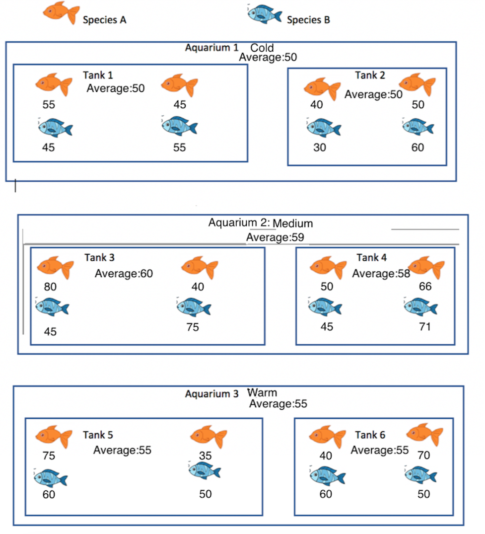
Figure 5.2: Fish in Aquarium Study
The first 10 rows of the dataset are shown below.
Fish <- 1:24
Tank <- factor(c(rep(1, 4), rep(2, 4), rep(3, 4), rep(4, 4), rep(5, 4), rep(6, 4)))
Aquarium <- c(rep(1, 8), rep(2, 8), rep(3, 8))
Species <- c("A","A","B","B","A","A","B","B","A","A","B","B","A","A","B","B","A","A","B",'B',"A","A","B","B")
Temp <- c(rep("Cold", 8), rep("Medium", 8), rep("Warm", 8))
Size <- c(rep(c("Large", "Large", "Small", "Small"),3))
Activity <- c(55, 45, 45, 55, 50, 50, 40, 60, 80, 40, 45, 75, 50, 66, 45, 71, 75, 35, 60, 50, 40, 70, 60, 50)
Activity <- c(60, 50, 40, 40, 50, 50, 40, 60, 80, 40, 45, 75, 50, 66, 45, 71, 80, 40, 65, 55, 35, 65, 55, 45)
FishData <- data.frame(Fish, Tank, Aquarium, Species, Temp, Size, Activity)
head(FishData, 10)
## Fish Tank Aquarium Species Temp Size Activity
## 1 1 1 1 A Cold Large 60
## 2 2 1 1 A Cold Large 50
## 3 3 1 1 B Cold Small 40
## 4 4 1 1 B Cold Small 40
## 5 5 2 1 A Cold Large 50
## 6 6 2 1 A Cold Large 50
## 7 7 2 1 B Cold Small 40
## 8 8 2 1 B Cold Small 60
## 9 9 3 2 A Medium Large 80
## 10 10 3 2 A Medium Large 4028) Identify the levels of a three-level experiment and the observational units and variables at each level.
Identify the levels of the data and list the observational unit and variable(s) measured at each level of the data.
29) Interpret fixed and random effects and associated parameter estimates in models with three or more levels.
For parts (a)-(b), let \(Y_{ijk}\) represent the activity level of a fish, where \(i\) indexes aquarium, \(j\) indexes tank, and \(k\) indexes fish. Suppose we fit a model of the form.
\(Y_{ijk} = \beta_{0} + a_{i}+t_{ij}+\epsilon_{ijk}\), where \(a_{i}\sim N(0,\sigma^2_a)\), \(t_{ij}\sim N(0,\sigma^2_t)\), and \(\epsilon_{ijk}\sim N(0,\sigma^2)\).
Explain in words what \(\beta_0\), \(\sigma_a\), \(\sigma_t\), and \(\sigma\) represent in this context.
Based on the activity levels shown in the illustration, which of \(\sigma_a\), \(\sigma_t\), and \(\sigma\), is the largest? Which is the smallest? Explain your answers.
Now suppose we fit a model of the form
\(Y_{ijk} = \beta_{0} +\beta_1\textrm{SpeciesB}_{ijk} + a_{i}+t_{ij}+\epsilon_{ijk}\), where \(a_{i}\sim N(0,\sigma^2_a)\), \(t_{ij}\sim N(0,\sigma^2_t)\), and \(\epsilon_{ijk}\sim N(0,\sigma^2)\).
Explain in words what \(\beta_0\), \(\sigma_a\), \(\sigma_t\), and \(\sigma\) represent in this context. In your answers state clearly how these interpretations are different than for the model in (a).
30) Write equations for linear mixed effects models in mathematical notation, including assumptions about distributions of random effects and error terms for models with three or more levels.
Write the mathematical notation of each of the following models, specified in R. Include appropriate subscripts and state the distributions of all random effects and error terms.